Diffusion models and time reversal

I recently spent some time reading about the algorithms behind Stable Diffusion and similar image generation models. They have been linked with an interesting 40-years-old result on diffusion processes¹. In short, this result states that there exists an explicit path from an initial probability distribution $p_0$ to a random noise (a normal distribution), and that this path can be reversed.

One application of this concept is sampling : we can draw a sample from a random noise and use the backward diffusion to obtain a sample from $p_0$. In the context of computer vision, this distribution would be multivariate with dimension $3 \times W \times H$, where $W$ and $H$ are respectively the width and height of a RGB image in pixels. The initial release of Stable Diffusion was using $H=W=512$.

In this document, I'll delve into the mechanics of reverse-time diffusions in dimension 1 (one pixel, one color channel) and derive equations to build a better understanding and intuition.

Forward diffusion#

The transition from an image to noise is accomplished by repetitively introducing random perturbations to our initial distribution. This can be done in a continuous time setting using an Ornstein-Uhlenbeck stochastic process. The Ornstein-Uhlenbeck process is defined by the following stochastic differential equation (SDE) :

where $W$ is a Brownian motion defined on some probability space $(\Omega, \mathcal{F}, P)$. The first term is forcing the mean to converge to $\mu$, while the second term is adding noise.

We can show using Itô's formula with $f(t, x) = x e^{\theta t}$ that

This means that the marginals of $X$ conditional to $X_0$ follow a normal distribution

We note that the mean tends to $\mu$, and the variance to $\sigma^2/(2\theta)$. We can then reparameterize the SDE such that the distribution of $X$ converges to a standard normal distribution (with unit variance) :

and :

At this point we can notice a few things :

• Impact of the noise level $\sigma$ : the noise (or volatility) parameter $\sigma$ has a similar impact on the diffusion as the time $t$. Increasing $\sigma$ will lead to noise being added faster
• Distribution of $X$ : the distribution of $X$ given $X_0$ is normal, but the unconditional distribution is not in general. In the case where $X_0$ is itself normal, each step of the diffusion will generate a new normal distribution as we sum independant Gaussian variables together

Backward diffusion#

We follow the notations of Haussmann and Pardoux² and define $Y_t = X_{1-t}$ for $0 \leq t \leq 1$. It can be shown¹² that the reverse process $Y$ follows the SDE

where

is the score function associated with distribution $p_{t}$ (derivative of its logarithm) and $\overline{W}$ another Brownian motion. In practice, the score is intractable and needs to be approximated.

Score matching#

One method is score matching³⁴. The score function $s_t$ is approximated using a parametrical model $s_\theta$ :

The $1/2$ constant is only a convention. We can simplify this expression by using an integration by part trick⁵. First we develop $J$ :

Since the last term does not depend on $\theta$, minimizing the rest will suffice. Thus our new cost function $\tilde{J}$ reads, after integration by part :

This removes the dependency to an explicit formulation of the distribution $p_t$. Instead we can rely on Monte-Carlo estimation for instance to compute the cost function.

Note 1 : $s_\theta = 0$ is the best constant model, but is beaten by linear models with negative slope. Indeed, the second term pushes the derivative of the score to be negative. This is consistent with the Gaussian case.

Note 2 : In dimension $N > 1$, the formulation becomes⁵ :

Neural networks are used in practice, where $\theta$ represents the weights of the network. The U-Net⁶ architecture for instance is used to estimate the score function in computer vision⁷.

Gaussian mixtures#

Another method would be to actually approximate the distribution $p_t$ with a Gaussian mixture. In this case, the score is explicit, which is a nice property. The drawback of this method is probably that the space of Gaussian mixtures is restrictive in some sense.

Centered Gaussian case#

When the initial distribution is Gaussian, the process $X$ stays Gaussian, and we get a closed form for the distribution $p$. We can then derive explicitely the reverse process.

Note : going from a normal distribution to a standard normal distribution can be done in one step : $X_1 = (X_0 - \mu) / \sigma$. The following derivation is for learning purpose only!

When $X_0 \sim \mathcal{N}(0, \sigma_0^2)$ we get

In this case the score function is

and the reverse SDE reads

where

Some interesting cases :

• $\sigma_0 = 1$ yields the forward SDE, which is expected since the initial and target distributions are the same in this case
• $\sigma_0^2 < 2$ means the mean reversion speed is always positive, while when $\sigma_0^2 \geq 2$, it can change sign during diffusion
• $\sigma_0 = 0$ leads to a SDE that starts as the forward SDE and tends to a singularity as $\alpha_{1-t}$ approaches 1. Indeed, the SDE cannot converge to a constant, as an independent noise is added at each step

The backward diffusion is an Ornstein-Uhlenbeck process with time dependent parameters. Using Itô's formula again with $f(t, x) = x e^{\frac{\sigma_0^2}{2}\int_0^t \beta_s ds}$, we get :

By rewriting $\beta_t$ as

one can recognize the derivative of a logarithm and find that

which tends to $0$ as $t \rightarrow 1$. This means that the variance contribution of the firm term is zero. The variance of the second term is more involved but leads to :

where $\gamma = 1 - \sigma_0^2$, which tends to

as $t \rightarrow 1$. Finally, we notice that this expression tends to $\sigma_0^2$ if $\sigma$ is sufficiently high. Similarly, we could have used $T > 1$ for a fixed $\sigma$, and let $T$ tend to infinity. As previously mentioned, noise level and time play similar roles.

Something interesting to note is that for a given level of convergence of the variance in the forward SDE, that is $\alpha_1 = \epsilon$, the variance of the reverse process will either converge faster or slower relative to $\sigma_0^2$ depending on the sign of $\gamma$. When the initial distribution has more variance than the random noise, the backward SDE will converge slower and vice versa.

PyTorch implementation#

We consider a 1-dimensional distribution $p$, and use the previous diffusion to generate a random noise. In order to target an end variance of $1 - \varepsilon$, we let $T = 1$ and $\sigma$ such that $\alpha_T = \varepsilon$. We use the Euler scheme to discretize the diffusion.

import math
 
import torch
 
 
NB_PATHS = 50
NB_TIMESTEPS = 100
T = 1.0
EPS = 0.001
 
 
def forward_diffusion_step(
    X: torch.Tensor,
    Z: torch.Tensor,
    sigma: float,
    dt: float,
) -> torch.Tensor:
    return X - 0.5 * sigma * sigma * X * dt + sigma * Z * math.sqrt(dt)
 
 
dt = T / NB_TIMESTEPS
sigma = math.sqrt(-math.log(EPS) / T)  # alpha_T = eps
X0 = torch.normal(0, 1, size=(NB_PATHS,))
X = torch.zeros((NB_TIMESTEPS, NB_PATHS))
Z = torch.normal(0, 1, size=(NB_TIMESTEPS - 1, NB_PATHS))
X[0] = X0
for i in range(NB_TIMESTEPS - 1):
  X[i+1] = forward_diffusion_step(X[i], Z[i], sigma, dt)

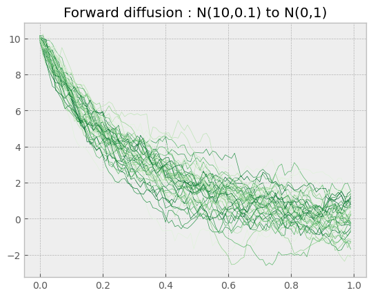
Here is a forward diffusion from $\mathcal{N}(10, 0.1)$ to $\mathcal{N}(0, 1)$ :

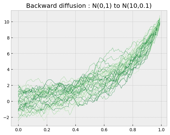
We write backward diffusion with score function in the normal case $\mathcal{N}(\mu_0, \sigma_0^2)$

def backward_diffusion_step(
    X: torch.Tensor,
    Z: torch.Tensor,
    sigma: float,
    mu0: float,
    sigma0: float,
    dt: float,
    t: float,
) -> torch.Tensor:
    sigma2 = sigma * sigma
    alpha = math.exp(-sigma2 * (1 - t))
    score = -(X - mu0 * math.sqrt(alpha)) / (sigma0 * sigma0 * alpha + 1 - alpha)
    return (
        X
        + 0.5 * sigma2 * X * dt
        + score * sigma2 * dt
        + sigma * Z * math.sqrt(dt)
    )

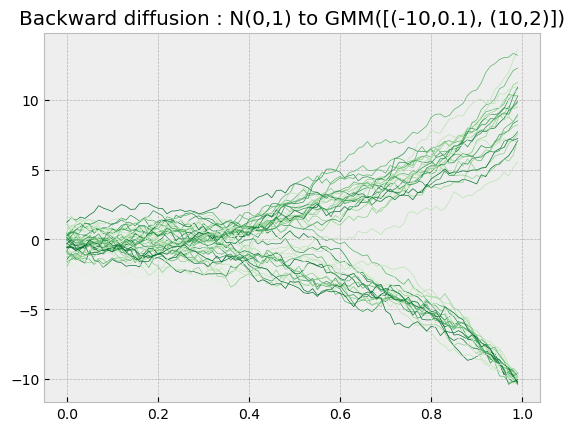
Finally, we can re-write the score used in the backward SDE when the initial distribution is a Gaussian mixture. Indeed, Gaussian mixtures are stable by addition with a normal variable, and we can proceed similarly to the previous case.

def backward_diffusion_step(
    X: torch.Tensor,
    Z: torch.Tensor,
    sigma: float,
    params0: List[Tuple[float, float]],
    t: float,
    dt: float,
) -> torch.Tensor:
    sigma2 = sigma * sigma
    alpha = math.exp(-sigma2 * (1 - t))
    n = len(params0)
    score, divisor = 0, 0
    for (mu0, sigma0) in params0:
        mut = mu0 * math.sqrt(alpha)
        sigmat2 = sigma0 * sigma0 * alpha + 1 - alpha
        denominator = math.sqrt(2 * math.pi * sigmat2)
        pit = np.exp(-(X - mut) * (X - mut) / (2 * sigmat2)) / denominator
        divisor += 1 / n * pit
        score -= 1 / n * pit * (X - mut) / sigmat2
    score /= divisor
    return (
        X
        + 0.5 * sigma2 * X * dt
        + score * sigma2 * dt
        + sigma * Z * math.sqrt(dt)
    )

That's all for today! ✨